Model hyperparameter optimization pipeline with Apache Airflow & Docker Swarm/Kubernetes

Introduction

Apache Airflow is a well known product for creating automated ETL (Extract-transform-load) pipelines to process raw data for training machine learning models. Similarly, Docker Swarm and Kubernetes are popular as management systems of containerized applications with multi-node/multi-cluster architectures.

In this post, we make use of these products together to create a model hyperparameter optimization pipeline that is easily scalable across many machines with one or more GPUs for accelerated computation. We need the system to have the following features:

1. Ability to create a workflow graph so that the pipeline task dependencies can be clearly seen and controlled
2. Ability to easily add and remove nodes (with GPU devices) before/during training
3. Have pre-training tasks that have functions like uploading raw data into an annotation tool, waiting for labeling to finish, transforming annotated data in the format suitable for consumption by our model trainer etc
4. Have a set of training and evaluation tasks that can train with different hyperparameters and different shuffled dataset sets
5. Have post-training tasks that carry out functions like determining the best model based on calculated test metrics and uploading as well as versioning the weights file of this model to production
6. Ability to monitor and report the status of each of the above tasks

This post uses the following versions of software:

• Apache Airflow – 2.2.4
• Docker – 20.10.16
• Kubernetes – 1.24.0

Additionally, we are referring to NVIDIA GPUs when GPUs are mentioned.

Designing the pipeline

Setting up

We can start designing our pipeline with Apache Airflow. To setup Airflow, we basically have two options – either install it locally or use docker images from DockerHub. If we intend to use Kubernetes for running and maintaining our pipeline, the former is advisable. On the other hand, if we want to stick with single machine or limited node architecture, the latter is better suited. Upgrading Airflow image version and avoiding dependency conflicts is much easier with docker images but then we will have to deal with docker-in-docker problems, i.e. when the Airflow inside the docker wants to control containers/nodes management tool (like Kubernetes and Docker) running on the host machine.

DAGs for pipeline

We can group all our tasks into three different cliques – which we will refer as DAGs (directed acyclic graph). Grouping tasks into DAGs not only makes the whole pipeline management much easier but also allows us to skip a set of tasks if we didn’t want them to run. For instance, if we already had labeled data, we would want to skip all the tasks responsible for labeling raw data. This would be much easier to do if we grouped labeling data into one DAG and similarly one each for others as appropriate.

The first one will be called Prelabeling DAG for handling data labeling, the second Training DAG will be responsible for finding the best set of hyperparameters and, lastly, Deployment DAG will handle the deployment of weights to production server.

Tasks in DAGs

For our use case of hyperparameter optimization, the prelabeling and deployment DAGs are better suited to be implemented in one node (we will refer as master node) while the training DAG is suited to be running dynamically one or more nodes (we will refer as worker nodes). This architecture minimizes complexity while still allowing the most work heavy part of our pipeline, i.e. training with different hyperparameters, to be parallelized across all the GPU devices we have. A short note regarding training parallelization we implement here is that, we want to parallelize each experiment as a whole by assigning it to a worker node rather than operator parallelization where training operations in one experiment are parallelized across several nodes. The latter form of parallelization brings another level of complexity which might not be worth dealing with in most applications.

Dashboard for recording experiment results

Tensorboard, generally, is the de-facto training dashboard for single machine training but if we want to train across different node that may also span different physical locations, using a cloud-based dashboard service might be more appropriate. Neptune.ai is one such solution I have used personally, among many other choices that are available.

Training Abstraction Layer (TAL)

Airflow is not designed to run a single task synchronously with the whole pipeline. This makes Airflow tasks unsuitable for creating a service for training tasks to communicate with to do things like abstracting away specific training dashboard, timing different parts of the training code, determining best validation and test results, managing model weights etc. To mitigate this, we can create a separate container/pod that runs a Training Abstraction Layer Service. The API calls exposed by this service can be implemented using something like XMLRPC for simplicity and each training experiment can be identified with an integer, we can call experiment_id, in every API function call parameter list.

The following are some example APIs that may be exposed by TAL:

def initialize_experiment(experiment_id: int, experiment_name: str, hyperparameters: Dict[str, Union[str, float, int]])
def end_experiment(experiment_id: int, failed: bool)

def notify_train_epoch_start(experiment_id: int, epoch: int, lr: float, _timestamp: float)
def notify_train_epoch_end(experiment_id: int, epoch: int, losses: Dict[str, float], _timestamp: float)

def notify_train_step_start(experiment_id: int, epoch: int, step: int, batch_size: int, _timestamp: float)
def notify_train_step_end(experiment_id: int, epoch: int, step: int, batch_size: int, _timestamp: float)

def notify_test_step_start(experiment_id: int, step: int, batch_size: int, _timestamp: float)
def notify_test_step_end(experiment_id: int, step: int, batch_size: int, _timestamp: float)

def notify_val_results(experiment_id: int, epoch: int, losses: Dict[str, float], metrics: Dict[str, float], _timestamp: float)
def notify_test_results(experiment_id: int, losses: Dict[str, float], metrics: Dict[str, float], _timestamp: float)

def notify_final_model_saved(experiment_id: int, weights_filename: str, _timestamp: float)

Interfacing training code with TAL and training tasks

If TAL APIs are implemented as XMLRPC server, the training code running in tasks will need to setup themselves as a XMLRPC client to call these functions. One important feature of XMLRPC is that it allows us to support function call batching. This kind of batching might be useful for API call pairs like notify_test_step_start/end listed above, as these call are usually made very fast adding cumulative network latencies to existing training latency.

One peculiar thing about the APIs defined above is that there is an extra _timestamp parameter to all the notify_ prefixed functions. This is because if we subtract timestamp between end and start of a step/epoch to time it on the server side, the calculated latency will also contain network latency with training code latency. Again, function batching will further degrade the accuracy of this timing calculation.

To solve this, we can create proxy layer code for TAL clients to use. This layer can automatically handle function batching and appending _timestamp for all notify_ calls for clients at the actual time of their call and so ensuring correctness.

Finally, we need the training code in repo to include a file containing a ‘list of hyperparameters’ so that the Airflow task responsible for creating experiments can pick one hyperparameter set from this file and dispatch a Airflow training task each. Similarly, the code in training repo should also be able to accept hyperparameter to train with using command line arguments.

Getting notification for task failure

Airflow supports setting DAG success and failure callbacks using on_success_callback and on_failure_callback. In these callbacks, we can use Airflow native operators like SlackWebhookOperator and EmailOperator to send Slack messages and email during DAG events we want to monitor.

System Architecture

The following diagram shows the full architecture of the proposed system. The master node runs the DAGs responsible for prelabeling and deployment while the worker nodes run training tasks from training DAG. Depending on the number of GPU devices available in each node, a node may take up multiple queued training tasks and run multiple trainings concurrently.

Because master and worker nodes are different machines, as shown in the figure below, they might need to share a storage mount point for reading and writing dataset and weights. To speed up training, a worker node might copy the dataset from the mount point to its local drive to avoid high latency if the mounted source is over a network. Again, when worker nodes finish their training, the mount point for weights will allow the master node to access and upload the best weight to production.

Finally, the Training Abstraction Layer (TAL), shown in the figure, runs in the master node and provides abstraction for worker node tasks as discussed in its section above.

Architecture

Implementing the pipeline

Prelabeling DAG

Prelabeling DAG would consist of the following:

• A task to fetch unannotated (raw) images from warehouse storage like Amazon S3 bucket to local disk
• A task to create tables and rows for training session and information about raw images
• A task to start a labeling session with a project ID in an annotation tool like CVAT
• A task to monitor the status of the labeling session
• A task to invoke the next DAG (training DAG) with project ID of the labeling session

Prelabeling DAG

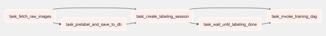
Annotation tools like CVAT report the completion status of labeling project by a status flag in their JSON response. For creating tasks that continuously pool this flag without wasting system resources (like a normal Python operator task would), we could use Airflow’s Deferred Operators. Again, running this DAG in a single node with its tasks as Celery workers should be the optimal implementation.

Deployment DAG

What deployment DAG does exactly might vary greatly depending on how a specific production environment is setup. But, generally, it would consist of the following:

• A task to report end of experiments and the best model via Slack, email etc
• A task to deploy the best model found with training experiments to production server

Deployment DAG

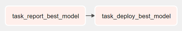
Just like in Prelabeling DAG, implementing these tasks as Celery workers seems like the most optimal method of implementation for the tasks in this DAG too. As to deploying to production server, we can either use a simple S3 bucket with custom versioning or make use of existing frameworks such as Tensorflow Serving. We probably want to manually invoke this DAG rather than automatically after Training DAG finishes.

Training DAG

The tasks in the training DAG should do the following:

• Download annotated data (identified by project ID in CVAT) from annotation tool
• Split dataset into training, validation and testing set
• Transform the dataset to the format suitable for training
• Create experiments from hyperparameters list file
• Run training and report test metrics via TAL APIs
• Determine the best model

One restriction of Apache Airflow is that tasks cannot be dynamically generated by other tasks and have to be determined at “compile” time of our DAG python script. This also means that the number of hyperparameter sets we can test must be a constant. One method of getting around this, implemented by task_check_empty_experiment in the figure for Training DAG below, is by a Python branch operator. If the number hyperparameters to test is less than the maximum number that we support (let’s say N), this branch operator can easily skip other training tasks that are not required.

Training DAG

Training and ranking strategy

If we just take the N experiments to test and determine the best model from them on just one shuffle of dataset using test metrices of the trained models, we run the risk of not getting the optimal best model as all the models tested have only seen that one set of dataset splits and so, we cannot be sure that the model selected this way hasn’t overfitted this set.

To mitigate this, we can do K shuffles of data and then do L experiments on each of them. This will lead to KxL number of experiments. Unfortunately, this number can get large pretty quick and hence is impractical. Rather, we can do is, first, determine N best model from M experiments with one shuffle of data. This is shown by find_best_N_models (implemented under an Airflow Task Group) in the figure above. Then, we do X epochs where we shuffle dataset to create a new set and rank the best N models found earlier, shown by find_top_model. The top model found this way will have to rank the best in three out of four experiments and hence we can be more confident about the ranking of our model.

Single machine training

If we are only going to use one machine with one GPU, running the pipeline becomes very simple. We simply run Airflow in a docker using their Docker Compose file at https://airflow.apache.org/docs/apache-airflow/<AIRFLOW_VERSION>/docker-compose.yaml. For the Airflow instance in the docker to be able to control the host docker, rather than directly changing the host machine’s file permission for /var/run/docker.sock and mapping it to the container, we can use docker service like bobrik/socat to proxy the access to the host file.

Again, as the dependency for training task i+1 is i to queue for this one GPU, they run one after another without any parallelization and need for synchronization. If there are more than one GPU and would like to queue our training tasks among them, however, we would probably want to have a similar setup as multi-machine training as discussed in the following sections.

To make sure that Airflow training task containers can access (NVIDIA) GPUs, we need to:

1. Install nvidia-docker2 and set default docker runtime to nvidia by editing /etc/docker/daemon.json.
2. Derive training task container images from nvidia/cuda:<CUDA_VERSION>-cudnn<CUDNN_VERSION>-runtime-ubuntu<UBUNTU_VERSION>.

Multi-machine training using Docker Swarm

Docker Swarm allows us to build upon the single machine training setup mentioned above and create a muti-node training setup with minimal effort. We create a master node (called manager) using docker swarm init --advertise-addr <MANAGER_IP>. Then, worker nodes can notify the master node that they want to join the swarm using docker swarm join --token <TOKEN> <MANAGER_IP>. Similarly, a worker node can leave the swarm using docker swarm leave. Until Docker Compose version 3, specifying container placement (under deploy block) is not supported. So, we will have to create manager and worker node in a swarm manually. Finally, we use Airflow’s DockerSwarmOperator to put training tasks to run on worker nodes.

Problems with Docker Swarm and its support in Airflow

Unfortunately, as of the date of this post, GPU support in Docker Swarm seems immature (i.e. not easy as in Kubernetes) and Airflow’s DockerSwarmOperator doesn’t support setting GPU resource constraint via its function parameters. The former can fixed with some work by referring to https://docs.docker.com/config/containers/resource_constraints. But the latter will require actually modifying Airflow code. We need to set resource constraints so that we can assign one training task to one GPU, if a node has multiple GPUs in it. Again, there seems to be a bug in Airflow version 2.2.4 where completion status for a Docker Swarm task cannot be properly determined by Airflow if enable_logging is enabled.

(Massive) multi-machine training using Kubernetes cluster

Given the problems with Docker Swarm and its integration with Airflow, we might have to stick with Kubernetes even if we wanted to create a simple GPU-based multi-node setup. Kubernetes was a large set of components to setup and manage a multi-cluster, multi-node production environment. For our use case, we might only need few of the components as we are not creating a customer facing production environment.

Generally, Kubernetes users might use a separate third-party tools like kind, minikube etc to setup heir Kubernetes cluster. These tools provide abstraction over native Kubernetes tools like kubeadm and kubectl. Airflow internally uses these native Kubernetes tools to create, manage and delete pods for its tasks. So, if we are running Airflow in a docker, we will need to map Kubernetes config file (usually located in ~/.kube/config), network plugin CNI file (example: for flannel it would be /run/flannel/subnet.env) and install Kubernetes in the container with Airflow. This approach may not provide the best experience, however.

This is because when a Kubernetes cluster is created on the host and Docker is a separate technology to Kubernetes. Instead, we could deploy Airflow in a Kubernetes cluster’s pod running on the master machine and notify Airflow about this by setting AIRFLOW__KUBERNETES__IN_CLUSTER to true.

Next, we will need to use KubernetesPodOperator for training tasks so that Kubernetes Executor picks them up to run across worker nodes while other tasks default to Celery so that they run on master node. We also need to set the executor argument of training task as kubernetes and AIRFLOW__CELERY_KUBERNETES_EXECUTOR__KUBERNETES_QUEUE must be set to kubernetes to use Kubernetes Executor properly. Finally, to enable NVIDIA GPU support for Kubernetes we will need to install NVIDIA device plugin.

Now that we have Airflow and Kubernetes master node running, we can make worker nodes join this cluster using kubedm join <MASTER_IP> --token <TOKEN> --discovery-token-ca-cert-hash <CA_CERT_HASH>.

Queuing training tasks among available GPU resources

Besides making parallelization among nodes easier when each node has just one GPU to use, Kubernetes, using its resource constraint feature, allows us to schedule more than one task in nodes which have more than one GPU. We can make use of this feature easily using KubernetesPodOperator‘s resources function argument. We can specify the minimum number of GPUs our training code needs using data structure of type kubernetes.client.models.V1ResourceRequirements for this function argument.

Extras: Port forwarding for WSL2 setup

If you have setup your master and worker nodes with Kubernetes/Docker in WSL2, you will need to setup port forwarding from WSL VM to host using the following PowerShell script as Administrator with the following:

For Docker Swarm:

$WSL_IP_ADDRESS=$args[0]
netsh interface portproxy add v4tov4 listenport=2377 listenaddress=0.0.0.0 connectport=2377 connectaddress=$WSL_IP_ADDRESS
netsh interface portproxy add v4tov4 listenport=7946 listenaddress=0.0.0.0 connectport=7946 connectaddress=$WSL_IP_ADDRESS
netsh interface portproxy add v4tov4 listenport=4789 listenaddress=0.0.0.0 connectport=4789 connectaddress=$WSL_IP_ADDRESS

For Kubernetes:

$WSL_IP_ADDRESS=$args[0]
netsh interface portproxy add v4tov4 listenport=6443 listenaddress=0.0.0.0 connectport=6443 connectaddress=$WSL_IP_ADDRESS
netsh interface portproxy add v4tov4 listenport=2379 listenaddress=0.0.0.0 connectport=2379 connectaddress=$WSL_IP_ADDRESS
netsh interface portproxy add v4tov4 listenport=2380 listenaddress=0.0.0.0 connectport=2380 connectaddress=$WSL_IP_ADDRESS
netsh interface portproxy add v4tov4 listenport=10250 listenaddress=0.0.0.0 connectport=10250 connectaddress=$WSL_IP_ADDRESS
netsh interface portproxy add v4tov4 listenport=10259 listenaddress=0.0.0.0 connectport=10259 connectaddress=$WSL_IP_ADDRESS
netsh interface portproxy add v4tov4 listenport=10257 listenaddress=0.0.0.0 connectport=10257 connectaddress=$WSL_IP_ADDRESS

TensorFlow v2+Keras re-implementation of ‘Old Photo Restoration via Deep Latent Space Translation’, CVPR 2020 paper

This is a TensorFlow v2+Keras inference ONLY implementation of a CVPR 2020 paper that restores old photos suffering from degradations like faded colors, scratches and color spots by jointly learning from the latent spaces of paired artificially degraded images and real degraded photos.

GitHub repo: https://github.com/sanje2v/OldPhotoRestorationDLST

Implementation of ‘Dual Super Resolution Learning For Semantic Segmentation’, CVPR 2020 paper

Abstract from paper: Current state-of-the-art semantic segmentation methods often apply high-resolution input to attain high performance, which brings large computation budgets and limits their applications on resource-constrained devices. In this paper, we propose a simple and flexible two-stream framework named Dual Super-Resolution Learning (DSRL) to effectively improve the segmentation accuracy without introducing extra computation costs. Specifically, the proposed method consists of three parts: Semantic Segmentation Super-Resolution (SSSR), Single Image Super-Resolution (SISR) and Feature Affinity (FA) module, which can keep high-resolution representations with low-resolution input while simultaneously reducing the model computation complexity. Moreover, it can be easily generalized to other tasks, e.g., human pose estimation. This simple yet effective method leads to strong representations and is evidenced by promising performance on both semantic segmentation and human pose estimation. Specifically, for semantic segmentation on CityScapes, we can achieve 2% higher mIoU with similar FLOPs, and keep the performance with 70% FLOPs. For human pose estimation, we can gain 2% mAP with the same FLOPs and maintain mAP with 30% fewer FLOPs.

---

GitHub repo: https://github.com/sanje2v/DualSuperResLearningForSemSeg

Accelerating data transforms

Deep learning training make use of data augmentation to expand the training set. In PyTorch and TensorFlow, these are called data transformers. As these transformers can be executed hundreds of thousands of times during training, it can be very beneficial to take some time to find ways to optimize them to their fastest versions. Hence, training time can be cut down by hours.

This short article shows two examples of transforms which you would think should already be the most optimal but are surprisingly not. The reported execution times are for segmentation map and image of sizes 2048×1024 px.

Remapping class label to training ids

This type of transformation can be found in segmentation tasks where we need to remap class labels to train ids because some class labels are not to be evaluated. We can accelerate the naive python implementation with ‘Numba‘ library where we compile python function to a fast implementation and also parallelize it.

# Naive implementation
def remapClassLabelsToTrainIds(segmentation_map, label_mapping_dict):
  for key, value in label_mapping_dict.items():
    segmentation_map[segmentation_map == key] = value

# Accelerated implementation
@numba.jit(nopython=True, parallel=True, cache=True, inline='always')
def remapClassLabelsToTrainIds(segmentation_map, label_mapping_dict):
  for row in numba.prange(segmentation_map.shape[0]):
    for col in numba.prange(segmentation_map.shape[1]):
      segmentation_map[row, col] = label_mapping_dict[segmentation_map[row, col]]

Naive implementation required around 100 milliseconds.

Accelerated implementation required around 400 milliseconds for "warmup" first call to compile for accelerated code and then afterwards required only 25 milliseconds. This makes the new implementation 4 times faster.

Hue shift (as seen in TorchVision 0.8)

The default hue shifting implementation from PyTorch+TorchVision is in ‘ColorJitter‘ class that does a RGB->HSV->Hue shift->RGB. This is an expensive chain of operations with memory copies that could have been avoided. The following code block shows ‘ColorJitter2‘ class whose implementation avoids these expensive operations and also remains backwards compatible. The added new code for hue shift starts from line number 102.

# Inplace hue shift code was adopted from 'https://stackoverflow.com/questions/8507885/shift-hue-of-an-rgb-color'
import torch as t
import torchvision as tv
import torchvision.transforms.functional as F
import numpy as np
import numba as nb
import numbers
import random


class ColorJitter2(t.nn.Module):
  """Randomly change the brightness, contrast and saturation of an image.

  Args:
    brightness (float or tuple of float (min, max)): How much to jitter brightness.
      brightness_factor is chosen uniformly from [max(0, 1 - brightness), 1 + brightness]
      or the given [min, max]. Should be non negative numbers.
    contrast (float or tuple of float (min, max)): How much to jitter contrast.
      contrast_factor is chosen uniformly from [max(0, 1 - contrast), 1 + contrast]
      or the given [min, max]. Should be non negative numbers.
    saturation (float or tuple of float (min, max)): How much to jitter saturation.
      saturation_factor is chosen uniformly from [max(0, 1 - saturation), 1 + saturation]
      or the given [min, max]. Should be non negative numbers.
    hue (float or tuple of float (min, max)): How much to jitter hue.
      hue_factor is chosen uniformly from [-hue, hue] or the given [min, max].
      Should have 0<= hue <= 0.5 or -0.5 <= min <= max <= 0.5.
  """

  def __init__(self, brightness=0, contrast=0, saturation=0, hue=0):
    super().__init__()
    self.brightness = self._check_input(brightness, 'brightness')
    self.contrast = self._check_input(contrast, 'contrast')
    self.saturation = self._check_input(saturation, 'saturation')
    self.hue = self._check_input(hue, 'hue', center=0, bound=(-0.5, 0.5),
                   clip_first_on_zero=False)

  @t.jit.unused
  def _check_input(self, value, name, center=1, bound=(0, float('inf')), clip_first_on_zero=True):
    if isinstance(value, numbers.Number):
      if value < 0:
        raise ValueError("If {} is a single number, it must be non negative.".format(name))
      value = [center - float(value), center + float(value)]
      if clip_first_on_zero:
        value[0] = max(value[0], 0.0)
    elif isinstance(value, (tuple, list)) and len(value) == 2:
      if not bound[0] <= value[0] <= value[1] <= bound[1]:
        raise ValueError("{} values should be between {}".format(name, bound))
    else:
      raise TypeError("{} should be a single number or a list/tuple with lenght 2.".format(name))

    # if value is 0 or (1., 1.) for brightness/contrast/saturation
    # or (0., 0.) for hue, do nothing
    if value[0] == value[1] == center:
      value = None
    return value

  @staticmethod
  @nb.jit(nopython=True, parallel=True, cache=True, inline='always')
  def _accelerated_matmul(img, hue_rotation_matrix):
    for row in nb.prange(img.shape[-2]):
      for col in nb.prange(img.shape[-1]):
        img[0, row, col] = img[0, row, col] * hue_rotation_matrix[0, 0] + img[1, row, col] * hue_rotation_matrix[0, 1] + img[2, row, col] * hue_rotation_matrix[0, 2]
        img[1, row, col] = img[0, row, col] * hue_rotation_matrix[1, 0] + img[1, row, col] * hue_rotation_matrix[1, 1] + img[2, row, col] * hue_rotation_matrix[1, 2]
        img[2, row, col] = img[0, row, col] * hue_rotation_matrix[2, 0] + img[1, row, col] * hue_rotation_matrix[2, 1] + img[2, row, col] * hue_rotation_matrix[2, 2]

  @staticmethod
  def _rotate_hue(img, hue_rotation_matrix):
    hue_rotation_matrix = np.array(hue_rotation_matrix, dtype=img.numpy().dtype) # CAUTION: Important to keep data types to same type of float
    ColorJitter2._accelerated_matmul(img.numpy(), hue_rotation_matrix)
    return t.clip(img, min=0., max=1.)

  def forward(self, img):
    """
    Args:
      img (Tensor): Input image.

    Returns:
      Tensor: Color jittered image.
    """
    assert isinstance(img, t.Tensor), "BUG CHECK: Only 'torch.Tensor' type of 'img' is supported for now."

    fn_idx = t.randperm(4)
    for fn_id in fn_idx:
      if fn_id == 0 and self.brightness is not None:
        brightness = self.brightness
        brightness_factor = t.tensor(1.0).uniform_(brightness[0], brightness[1]).item()
        img = F.adjust_brightness(img, brightness_factor)

      if fn_id == 1 and self.contrast is not None:
        contrast = self.contrast
        contrast_factor = t.tensor(1.0).uniform_(contrast[0], contrast[1]).item()
        img = F.adjust_contrast(img, contrast_factor)

      if fn_id == 2 and self.saturation is not None:
        saturation = self.saturation
        saturation_factor = t.tensor(1.0).uniform_(saturation[0], saturation[1]).item()
        img = F.adjust_saturation(img, saturation_factor)

      if fn_id == 3 and self.hue is not None:
        hue = self.hue
        hue_factor = t.tensor(1.0).uniform_(hue[0], hue[1]).item()
        hue_factor_radians = hue_factor * 2.0 * np.pi

        # Prepare rotation matrix
        cosA = np.cos(hue_factor_radians)
        sinA = np.sin(hue_factor_radians)
        hue_rotation_matrix =\
          [[cosA + (1.0 - cosA) / 3.0, 1./3. * (1.0 - cosA) - np.sqrt(1./3.) * sinA, 1./3. * (1.0 - cosA) + np.sqrt(1./3.) * sinA],
           [1./3. * (1.0 - cosA) + np.sqrt(1./3.) * sinA, cosA + 1./3.*(1.0 - cosA), 1./3. * (1.0 - cosA) - np.sqrt(1./3.) * sinA],
           [1./3. * (1.0 - cosA) - np.sqrt(1./3.) * sinA, 1./3. * (1.0 - cosA) + np.sqrt(1./3.) * sinA, cosA + 1./3. * (1.0 - cosA)]]
        img = ColorJitter2._rotate_hue(img, hue_rotation_matrix)

    return img

  def __repr__(self):
    format_string = self.__class__.__name__ + '('
    format_string += 'brightness={0}'.format(self.brightness)
    format_string += ', contrast={0}'.format(self.contrast)
    format_string += ', saturation={0}'.format(self.saturation)
    format_string += ', hue={0})'.format(self.hue)
    return format_string

Naive implementation required around 240 milliseconds.

Accelerated implementation required around 800 milliseconds for "warmup" first call to compile for accelerated code and then afterwards required only 32 milliseconds. This makes the new implementation 7.5 times faster.

Conclusion

As we can see, even though accelerated implementations shown above take some extra time in their first call, they become very fast in latter calls. Hence, these will overtake naive implementations very quickly. Of course, the reported speedups will vary according to different systems but given how prevalent multi-core CPUs are, parallelization in accelerated implementation should provide good guarantee they will be faster across different systems.

Book summary: Learning From Data

Most of deep learning research nowadays is based around proposing newer models with larger number of parameters and novel methods with weak theoretical basis on why such a model could out perform its other competitive counterparts models. A large part of this is because of the inherent complexity in understanding the huge number of interactions among parameters in a deep learning model. So, studying theoretical basis of deep learning models have mostly been sidelined in favor of treating them as a black box and experimentally comparing performance among them in a leader board.

To begin mitigating this, ‘Learning from data – A short course‘ by Yaser S. Abu-Mostafa et al. is an important book in the sense that it tries to answer and provide a mathematical basis of learning problem in general – starting from the fundamental question of why it is possible to learn anything at all. The book is a great read for both amateurs and specialists of deep learning alike as the mathematical concepts required to digest the material is elementary. Yet for first time readers, the newness of materials covered might make the flow of the argument being made quite confusing. Hence, this post lists major bullet points on the important chapters (i.e. not all chapters are covered) for my own future reference and for anyone else who might benefit from a summary of this book with added notes of my own.

Chapter 1: The Learning Problem

1. Difference between Learning and Design approaches:
   • Learning approach uses data to search the hypothesis set for a good hypothesis that can correctly classify training data. The resultant hypothesis is then used to make predictions on out-of-sample data generated by the same unknown target function that generated the training data. Example: The problem of accepting or denying credit for a bank customer. As there are many factors (usually called features in a learning problems) affecting a customer’s ability to pay back debt, we have to analyze all previous data we have of him/her and similar customers to make a yes/no decision on granting further credit.
   • Design approach uses specifications (along with probability and statistics) to analytically define unknown target function without any need to see data. Example: The problem of classification of coins. As coins are produced by machines (also verified manually before distribution) with very little error on their diameter and form, a formal design specification with allowance for random error might be sufficient to classify them.
2. The book only deals with learning approaches and hence brief discussion on the types of learning methods:
   • Supervised learning: Training data consists of input and its corresponding output pair. The objective of a supervised learner is to be able to match input and output pair by computing errors in each training iteration and rearranging its internal configuration accordingly. Types of supervised learning are:
     1. Active learning: Here output for an input data can be queried from the training set. This allows us for strategic choice of inputs.
     2. Online learning: Here examples of training data arrives in a stream. So, the learner has no strategic choice of input and has to learn examples as they come.
   • Reinforcement learning: Training data consists of input, its corresponding output and a grade for the output. The data does not define how good other outputs would have been for other inputs. The grade for the output functions as a rewarding function that the learning is trying to maximize as it defines what the best course of action is.
   • Unsupervised learning: Training data consists of only input and so an unsupervised learner is tasked with finding patterns between input data points to categorize them into unlabelled clusters. The evaluation phase consists of correctly classifying out of sample data into one of these clusters.
3. We can create learners to memorize the training set by using very complex hypothesis with lot of parameters but can we create a learner from in-sample data to make predictions on out-sample data (generated by non-random target function)?
   • Deterministically – NO
   • Probabilistically – YES
4. Introduction to Bin Model: To establish statement (3) above, we first introduce an analogical problem called Bin Model where we model a bin with unknown (could even be infinite) number of red and green marbles. The problem is to bound the = probability of red marbles in the bin (so = probability of green marbles) with = fraction of red samples from = total marbles (with replacement) randomly sampled from the bin.
5. Hoeffding’s Inequality, , where is probability and is the threshold of error that correctly tracks . This inequality can help us bound the fraction of red marbles that are drawn
6. Notes for Hoeffding’s Inequality equation:
   • The inequality only holds if the samples are randomly drawn.
   • is a constant while is a random variable dependent on the value of .
   • The right side of the equation only has and . This implies that the bound is only dependent on how small the error threshold we choose is and the number of samples drawn but not on the number of samples in the bin. In fact, the number of samples in the bin could be infinite.
   • Larger the number of samples drawn from the bin, , better the probability that will track within error threshold.
7. Extension of bin model to one hypothesis: The bin framework can be reconstituted to establish statement (3) about learning for one hypothesis (for now) by redefining the red marbles as data points where hypothesis function does not match target function, i.e. , and vice versa for green marbles. For these redefinition to hold, we have to make sure that training inputs are randomly sampled according to a unknown probability distribution over input space .
8. Two rules from probabilities, given events , , …, :
   • If implies , then
   • Union Bound:
9. Extension of bin model to multiple hypothesis: Using rules from statement (7), we reconstitute statement (6) for multiple hypothesis as: where is in-sample error, is out-of-sample error, is final hypothesis, is the total number of hypothesis in the hypothesis set.
10. Notes about statement (8):
    • is infinite (for now) and hence the bounding is currently too weak to be of any use. This will be dealt with in the next chapter.
    • Depending on complexity different hypothesis, the bounds can be of different sizes but for simplification they are assumed to be of one size and hence equation (8) has instead of summation.
    • The equation seems to imply that a simple target function can be learned as easily a complex function with a simple hypothesis. This is because the statement only deals with trying to keep out-of-sample error close to in-sample error while not dealing with the requirement of making in-sample error small (see statement (10)). The complexity of a hypothesis deals with the latter.
11. Requirements for actual learning:
    • Out-of-sample error is close to in-sample error
    • In-sample error is small enough
12. Noisy data: Real world data is noisy. For this, we try to model instead, where noise is accommodated in and input samples are picked with an unknown distribution .

Chapter 2: Training versus Testing

1. Generalization bound: We can rewrite equation in Chapter 1, statement 9 to create a bound between and , as follows:
2. Reducing infinite hypothesis choices to polynomial: The term in Chapter 1, point 9 is infinite which makes the bound useless. Again, the union bound in Chapter 1, statement 8, consists of events that heavily overlap. This again makes this bound unnecessarily wide. To remedy this, we , first, recognize that given points for a model to learn to classify, there can only be a fixed number of dichotomies that a specific model can produce. We will call this bounding the growth function of a model. This bound will replace the infinite term with a polynomial. We will consider binary target function for simplicity but will later extend to real-valued functions.
3. Growth function: This function gives the maximum number of dichotomies that can be generated by a hypothesis set (created by a learning algorithm) on given points to classify. Mathematically, growth function
4. Break point: If no data set of size can be shattered (i.e. produce all possible dichotomies) by , then is said to be a break point for . If a model can shatter any then .
5. Need to bound growth function: If for a hypothesis (i.e. it is too complex), the generalization error term (from statement (1)) will never go to zero regardless of the number of training examples. Then, the model will memorize the training set instead of learning from it. On the other hand, bounding by any polynomial, will bring generalization error to zero when the number of samples .
6. Bounding growth function: Using recursive techniques, we find that if for some value , then . The RHS of the equation is a polynomial in of degree.
7. Vapnik-Chervonenkis Dimension: VC dimension is the largest for which . If for all N, . We redefine the equation in statement (6) with VC dimension as: . VC dimension can be thought of as measuring ‘effective’ parameters of a model to express a diverse set of hypothesis.
8. VC Generalization bound: Finally we replace in Generalization bound defined in statement (1) with VC Generalization Bound as: .
9. Notes on VC Generalization bound:
   • The slack in the bound can be attributed to: a) the bound being the same for different values of , b) Maximum number of dichotomies being considered, and c) is bounded by simple polynomial
   • Despite the bound being loose, it: a) establishes the feasibility of learning despite having infinite hypothesis set, and b) is equally loose for different learning models and hence allows generalized performance comparisons between them.
10. Sample complexity: Sample complexity is the number of training examples needed to achieve a certain generalization performance. We can estimate the number of training examples needed for generalization error to remain equal or less than is given by: . We can use iterative method to get for an error threshold .
11. Penalty for Model complexity: Higher model complexity (i.e. with higher VC dimension) is more like to fit training set but loose generalization in out-of-sample test set. An intermediate VC dimension (found through training and testing) will be the best level of model complexity with minimum out-of-sample error and low (but not minimum) in-sample error.
12. Test Set: A part of training data set kept aside for testing the final hypothesis after training is called test set. is considered synonymous to for practical purposes as technically cannot be calculated.
    • Because it has only the final hypothesis to calculate error against, its bound is much more strict than the bound with hypothesis set during training.
    • Larger test sets give more accurate estimate of . Though too a big of a test set, leads to too small of a training set which in turn degrades the ability of the model to learn anything.
    • When test set is not used in any form during training or to select the final hypothesis, a test set does not have a bias and only variance.
13. Extension from binary to real-valued functions: Bias-variance decomposition of out-of-sample error can be expressed as: .
14. Notes on bias-variance:
    • An ideal model has both low bias and variance.
    • Generally, trying to reduce bias increases variance and vice versa.
    • A good hypothesis, has an ‘acceptable’ compromise of bias and variance values.
    • In VC analysis, out-of-sample error is the sum of in-sample error and generalization error while in bias-variance analysis it is the sum of bias and variance.

Chapter 4: Overfitting

1. Effects of:
   • Increase in number of training data – Overfitting decreases
   • Increase in noise – Overfitting increases
   • Increase in target complexity – Overfitting increases
2. Types of noise:
   • Stochastic: This is the random noise in the data. This noise changes every time data is generated from the target function.
   • Deterministic: This noise comes from the complexity of the target function (not considering added random noise) as a model tries to fit approximate the target function with its complexity using the available degrees of freedom. This noise does not change is the same data is generated but different models can have different deterministic noises depending on their complexity (and parameters).
3. In bias-variance analysis in Chapter 2, statement 13:
   • Stochastic noise will be an addition parameter in the equation as: .
   • Deterministic noise is captured by bias in the equation while variance is effected by both types of noises.
4. Regularization: This reduces overfitting by limiting the degrees of freedom of model to selection of simpler hypothesis. The decision to whether to use regularization is heuristics-based. Regularization, generally, mildly increases bias while strongly reducing variance.
5. Validation Set: A test set is an unbiased estimate of and never used in training or in making choices in the learning process while a validation set, while not used in training directly, is used in certain choices in the learning process. Training with validation set data points, consists of first training with data points, validation with data points to estimate the model with best and then finally retraining with all data points to produce the final hypothesis.
6. Cross Validation: Setting aside too large of validation data points reduces the number of training samples while setting aside too small leads to be a weak estimate of . V-fold cross validation is one type of cross validation method, where training data is divided into disjoint sets each of size . Hence, training always happens on data not used for validation and the validation error is average of validation error in each . This allows cross validation to be more effective than just naive validation method.

Chapter 5: Three Learning Principles

1. Occam’s Razor: Simpler models generally produce lower out-of-sample errors. Hence, it is preferable to select a simpler hypothesis than a complex one.
2. Sampling Bias: If models are trained with a dataset which is sampled in a biased way, the resultant model will also be biased. One way to avoid this would be to train with multiple datasets.
3. Data Snooping: Looking at testing data to choose a learning model compromises the ability to properly learn as it affects the ability to assess outcome. A portion of testing data from total training set data must be set aside and not be used to in anything besides testing the final hypothesis.