
Most of deep learning research nowadays is based around proposing newer models with larger number of parameters and novel methods with weak theoretical basis on why such a model could out perform its other competitive counterparts models. A large part of this is because of the inherent complexity in understanding the huge number of interactions among parameters in a deep learning model. So, studying theoretical basis of deep learning models have mostly been sidelined in favor of treating them as a black box and experimentally comparing performance among them in a leader board.
To begin mitigating this, ‘Learning from data – A short course‘ by Yaser S. Abu-Mostafa et al. is an important book in the sense that it tries to answer and provide a mathematical basis of learning problem in general – starting from the fundamental question of why it is possible to learn anything at all. The book is a great read for both amateurs and specialists of deep learning alike as the mathematical concepts required to digest the material is elementary. Yet for first time readers, the newness of materials covered might make the flow of the argument being made quite confusing. Hence, this post lists major bullet points on the important chapters (i.e. not all chapters are covered) for my own future reference and for anyone else who might benefit from a summary of this book with added notes of my own.

Chapter 1: The Learning Problem
- Difference between Learning and Design approaches:
- Learning approach uses data to search the hypothesis set
- Design approach uses specifications (along with probability and statistics) to analytically define unknown target function without any need to see data. Example: The problem of classification of coins. As coins are produced by machines (also verified manually before distribution) with very little error on their diameter and form, a formal design specification with allowance for random error might be sufficient to classify them.
- Learning approach uses data to search the hypothesis set
- The book only deals with learning approaches and hence brief discussion on the types of learning methods:
- Supervised learning: Training data consists of input and its corresponding output pair. The objective of a supervised learner is to be able to match input and output pair by computing errors in each training iteration and rearranging its internal configuration accordingly. Types of supervised learning are:
- Active learning: Here output for an input data can be queried from the training set. This allows us for strategic choice of inputs.
- Online learning: Here examples of training data arrives in a stream. So, the learner has no strategic choice of input and has to learn examples as they come.
- Reinforcement learning: Training data consists of input, its corresponding output and a grade for the output. The data does not define how good other outputs would have been for other inputs. The grade for the output functions as a rewarding function that the learning is trying to maximize as it defines what the best course of action is.
- Unsupervised learning: Training data consists of only input and so an unsupervised learner is tasked with finding patterns between input data points to categorize them into unlabelled clusters. The evaluation phase consists of correctly classifying out of sample data into one of these clusters.
- Supervised learning: Training data consists of input and its corresponding output pair. The objective of a supervised learner is to be able to match input and output pair by computing errors in each training iteration and rearranging its internal configuration accordingly. Types of supervised learning are:
- We can create learners to memorize the training set by using very complex hypothesis with lot of parameters but can we create a learner from in-sample data to make predictions on out-sample data (generated by non-random target function)?
- Deterministically – NO
- Probabilistically – YES
- Introduction to Bin Model: To establish statement (3) above, we first introduce an analogical problem called Bin Model where we model a bin with unknown (could even be infinite) number of red and green marbles. The problem is to bound the
= probability of red marbles in the bin (so
= total marbles (with replacement) randomly sampled from the bin.
- Hoeffding’s Inequality,
is the threshold of error that
correctly tracks
- Notes for Hoeffding’s Inequality equation:
- The inequality only holds if the samples are randomly drawn.
- The right side of the equation only has
- Larger the number of samples drawn from the bin,
- Extension of bin model to one hypothesis: The bin framework can be reconstituted to establish statement (3) about learning for one hypothesis (for now) by redefining the red marbles as data points where hypothesis function does not match target function, i.e.
, and vice versa for green marbles. For these redefinition to hold, we have to make sure that
training inputs are randomly sampled according to a unknown probability distribution
over input space
.
- Two rules from probabilities, given events
,
, …,
:
- If
- Union Bound:
- If
- Extension of bin model to multiple hypothesis: Using rules from statement (7), we reconstitute statement (6) for multiple hypothesis as:
where
is in-sample error,
is out-of-sample error,
is final hypothesis,
is the total number of hypothesis in the hypothesis set.
- Notes about statement (8):
- Depending on complexity different hypothesis, the bounds can be of different sizes but for simplification they are assumed to be of one size and hence equation (8) has
- The equation seems to imply that a simple target function can be learned as easily a complex function with a simple hypothesis. This is because the statement only deals with trying to keep out-of-sample error close to in-sample error while not dealing with the requirement of making in-sample error small (see statement (10)). The complexity of a hypothesis deals with the latter.
- Requirements for actual learning:
- Out-of-sample error is close to in-sample error
- In-sample error is small enough
- Noisy data: Real world data is noisy. For this, we try to model


![\mathbb{P}[|\nu - \mu| > \epsilon] \leq 2e^{-2\epsilon^{2}N} \text{ for any } \epsilon > 0](https://s0.wp.com/latex.php?latex=%5Cmathbb%7BP%7D%5B%7C%5Cnu+-+%5Cmu%7C+%3E+%5Cepsilon%5D+%5Cleq+2e%5E%7B-2%5Cepsilon%5E%7B2%7DN%7D+%5Ctext%7B+for+any+%7D+%5Cepsilon+%3E+0&bg=ffffff&fg=393939&s=0&c=20201002)

![\mathbb{P}[\mathcal{B}_1] \leq \mathbb{P}[\mathcal{B}_2]](https://s0.wp.com/latex.php?latex=%5Cmathbb%7BP%7D%5B%5Cmathcal%7BB%7D_1%5D+%5Cleq+%5Cmathbb%7BP%7D%5B%5Cmathcal%7BB%7D_2%5D&bg=ffffff&fg=393939&s=0&c=20201002)
![\mathbb{P}[\mathcal{B}_1\text{ or }\mathcal{B}_2\text{ or ... or }\mathcal{B}_M] \leq \mathbb{P}[\mathcal{B}_1] + \mathbb{P}[\mathcal{B}_2] + ... + \mathbb{P}[\mathcal{B}_M]](https://s0.wp.com/latex.php?latex=%5Cmathbb%7BP%7D%5B%5Cmathcal%7BB%7D_1%5Ctext%7B+or+%7D%5Cmathcal%7BB%7D_2%5Ctext%7B+or+...+or+%7D%5Cmathcal%7BB%7D_M%5D+%5Cleq+%5Cmathbb%7BP%7D%5B%5Cmathcal%7BB%7D_1%5D+%2B+%5Cmathbb%7BP%7D%5B%5Cmathcal%7BB%7D_2%5D+%2B+...+%2B+%5Cmathbb%7BP%7D%5B%5Cmathcal%7BB%7D_M%5D&bg=ffffff&fg=393939&s=0&c=20201002)


Chapter 2: Training versus Testing
- Generalization bound: We can rewrite equation in Chapter 1, statement 9 to create a bound between
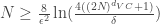
- Reducing infinite hypothesis choices to polynomial: The term
- Growth function: This function gives the maximum number of dichotomies that can be generated by a hypothesis set (created by a learning algorithm) on
- Break point: If no data set of size
- Need to bound growth function: If
- Bounding growth function: Using recursive techniques, we find that if
- Vapnik-Chervonenkis Dimension: VC dimension
- VC Generalization bound: Finally we replace
- Notes on VC Generalization bound:
- The slack in the bound can be attributed to: a) the bound being the same for different values of
- Despite the bound being loose, it: a) establishes the feasibility of learning despite having infinite hypothesis set, and b) is equally loose for different learning models and hence allows generalized performance comparisons between them.
- The slack in the bound can be attributed to: a) the bound being the same for different values of
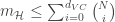
- Sample complexity: Sample complexity is the number of training examples needed to achieve a certain generalization performance. We can estimate the number of training examples needed for generalization error to remain equal or less than
- Penalty for Model complexity: Higher model complexity (i.e. with higher VC dimension) is more like to fit training set but loose generalization in out-of-sample test set. An intermediate VC dimension (found through training and testing) will be the best level of model complexity with minimum out-of-sample error and low (but not minimum) in-sample error.
- Test Set: A part of training data set kept aside for testing the final hypothesis after training is called test set.
- Because it has only the final hypothesis to calculate error against, its bound is much more strict than the bound with hypothesis set during training.
- Larger test sets give more accurate estimate of
- When test set is not used in any form during training or to select the final hypothesis, a test set does not have a bias and only variance.
- Extension from binary to real-valued functions: Bias-variance decomposition of out-of-sample error can be expressed as:
- Notes on bias-variance:
- An ideal model has both low bias and variance.
- Generally, trying to reduce bias increases variance and vice versa.
- A good hypothesis, has an ‘acceptable’ compromise of bias and variance values.
- In VC analysis, out-of-sample error is the sum of in-sample error and generalization error while in bias-variance analysis it is the sum of bias and variance.


![\mathbb{E}_{\mathcal{D}}[E_{out}(g^{(\mathcal{D})})] = \mathbb{E}_x[\text{bias}(x)]+\mathbb{E}_x[\text{var}(x)]](https://s0.wp.com/latex.php?latex=%5Cmathbb%7BE%7D_%7B%5Cmathcal%7BD%7D%7D%5BE_%7Bout%7D%28g%5E%7B%28%5Cmathcal%7BD%7D%29%7D%29%5D+%3D+%5Cmathbb%7BE%7D_x%5B%5Ctext%7Bbias%7D%28x%29%5D%2B%5Cmathbb%7BE%7D_x%5B%5Ctext%7Bvar%7D%28x%29%5D&bg=ffffff&fg=393939&s=0&c=20201002)
Chapter 4: Overfitting
- Effects of:
- Increase in number of training data – Overfitting decreases
- Increase in noise – Overfitting increases
- Increase in target complexity – Overfitting increases
- Types of noise:
- Stochastic: This is the random noise in the data. This noise changes every time data is generated from the target function.
- Deterministic: This noise comes from the complexity of the target function (not considering added random noise) as a model tries to fit approximate the target function with its complexity using the available degrees of freedom. This noise does not change is the same data is generated but different models can have different deterministic noises depending on their complexity (and parameters).
- In bias-variance analysis in Chapter 2, statement 13:
- Stochastic noise will be an addition parameter in the equation as:
- Deterministic noise is captured by bias in the equation while variance is effected by both types of noises.
- Stochastic noise will be an addition parameter in the equation as:
- Regularization: This reduces overfitting by limiting the degrees of freedom of model to selection of simpler hypothesis. The decision to whether to use regularization is heuristics-based. Regularization, generally, mildly increases bias while strongly reducing variance.
- Validation Set: A test set is an unbiased estimate of
- Cross Validation: Setting aside too large of
![\mathbb{E}_{\mathcal{D}}[E_{out}(g^{(\mathcal{D})})] = \sigma^2 + \mathbb{E}_x[\text{bias}(x)]+\mathbb{E}_x[\text{var}(x)]\text{ where }\sigma^2\text{ is variance of stochastic noise}](https://s0.wp.com/latex.php?latex=%5Cmathbb%7BE%7D_%7B%5Cmathcal%7BD%7D%7D%5BE_%7Bout%7D%28g%5E%7B%28%5Cmathcal%7BD%7D%29%7D%29%5D+%3D+%5Csigma%5E2+%2B+%5Cmathbb%7BE%7D_x%5B%5Ctext%7Bbias%7D%28x%29%5D%2B%5Cmathbb%7BE%7D_x%5B%5Ctext%7Bvar%7D%28x%29%5D%5Ctext%7B+where+%7D%5Csigma%5E2%5Ctext%7B+is+variance+of+stochastic+noise%7D&bg=ffffff&fg=393939&s=0&c=20201002)


Chapter 5: Three Learning Principles
- Occam’s Razor: Simpler models generally produce lower out-of-sample errors. Hence, it is preferable to select a simpler hypothesis than a complex one.
- Sampling Bias: If models are trained with a dataset which is sampled in a biased way, the resultant model will also be biased. One way to avoid this would be to train with multiple datasets.
- Data Snooping: Looking at testing data to choose a learning model compromises the ability to properly learn as it affects the ability to assess outcome. A portion of testing data from total training set data must be set aside and not be used to in anything besides testing the final hypothesis.


